Mutation Free Energy Calculations using BioExcel Building Blocks (biobb)
Based on the official pmx tutorial: http://pmx.mpibpc.mpg.de/sardinia2018_tutorial1/index.html
This tutorial aims to illustrate how to compute a fast-growth mutation free energy calculation, step by step, using the BioExcel Building Blocks library (biobb). The particular example used is the Staphylococcal nuclease protein (PDB code 1STN, https://doi.org/10.2210/pdb1STN/pdb), a small, minimal protein, appropriate for a short tutorial.
The non-equilibrium free energy calculation protocol performs a fast alchemical transition in the direction WT->Mut and back Mut->WT. The two equilibrium trajectories needed for the tutorial, one for Wild Type (WT) and another for the Mutated (Mut) protein (Isoleucine 10 to Alanine -I10A-), have already been generated and are included in this example. We will name WT as stateA and Mut as stateB.
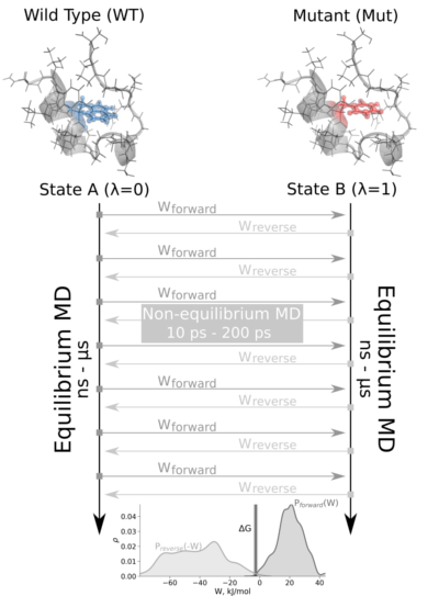
The tutorial calculates the free energy difference in the folded state of a protein. Starting from two 1ns-length independent equilibrium simulations (WT and mutant), snapshots are selected to start fast (50ps) transitions driving the system in the forward (WT to mutant) and reverse (mutant to WT) directions, and the work values required to perform these transitions are collected. With these values, Crooks Gaussian Intersection (CGI), Bennett Acceptance Ratio (BAR) and Jarzynski estimator methods are used to calculate the free energy difference between the two states.
Please note that for the sake of disk space this tutorial is using 1ns-length equilibrium trajectories, whereas in the original example the equilibrium trajectories used were obtained from 10ns-length simulations.
Biobb modules used
biobb_pmx: Tools to setup and run Alchemical Free Energy calculations.
biobb_gromacs: Tools to setup and run Molecular Dynamics simulations.
biobb_analysis: Tools to analyse Molecular Dynamics trajectories.
Auxiliary libraries used
Conda Installation and Launch
git clone https://github.com/bioexcel/biobb_wf_pmx_tutorial.git
cd biobb_wf_pmx_tutorial
conda env create -f conda_env/environment.yml
conda activate biobb_wf_pmx_tutorial
jupyter-notebook biobb_wf_pmx_tutorial/notebooks/biobb_wf_pmx_tutorial.ipynb
Pipeline steps:
Initializing colab
The two cells below are used only in case this notebook is executed via Google Colab. Take into account that, for running conda on Google Colab, the condacolab library must be installed. As explained here, the installation requires a kernel restart, so when running this notebook in Google Colab, don’t run all cells until this installation is properly finished and the kernel has restarted.
# Only executed when using google colab
import sys
if 'google.colab' in sys.modules:
  import subprocess
  from pathlib import Path
  try:
    subprocess.run(["conda", "-V"], check=True)
  except FileNotFoundError:
    subprocess.run([sys.executable, "-m", "pip", "install", "condacolab"], check=True)
    import condacolab
    condacolab.install()
    # Clone repository
    repo_URL = "https://github.com/bioexcel/biobb_wf_pmx_tutorial.git"
    repo_name = Path(repo_URL).name.split('.')[0]
    if not Path(repo_name).exists():
      subprocess.run(["mamba", "install", "-y", "git"], check=True)
      subprocess.run(["git", "clone", repo_URL], check=True)
      print("⏬ Repository properly cloned.")
    # Install environment
    print("⏳ Creating environment...")
    env_file_path = f"{repo_name}/conda_env/environment.yml"
    subprocess.run(["mamba", "env", "update", "-n", "base", "-f", env_file_path], check=True)
    print("👍 Conda environment successfully created and updated.")
# Enable widgets for colab
if 'google.colab' in sys.modules:
  from google.colab import output
  output.enable_custom_widget_manager()
  # Change working dir
  import os
  os.chdir("biobb_wf_pmx_tutorial/biobb_wf_pmx_tutorial/notebooks")
  print(f"📂 New working directory: {os.getcwd()}")
Workflow required files
Workflow Input files needed:
stateA_traj: Equilibrium trajectory for the WT protein.
stateB_traj: Equilibrium trajectory for the Mutated protein.
stateA_tpr: WT protein topology (GROMACS tpr format).
stateB_tpr: Mutated protein topology (GROMACS tpr format).
Auxiliary force field libraries needed:
mutff45 (folder): pmx mutation force field libraries.
Collected transitions work values:
dhdlA.zip: Forward work values required to illustrate how to perform the last step of the pmx workflow with real values, to extract the free energy.
dhdlB.zip: Reverse work values required to illustrate how to perform the last step of the pmx workflow with real values, to extract the free energy.
import os
import sys
import zipfile

cwd = os.getcwd()
# set prefix
prefix = '/usr/local' if 'google.colab' in sys.modules else os.getenv('CONDA_PREFIX')
gmxlib = prefix + '/lib/python3.10/site-packages/pmx/data/mutff/'

stateA_traj = cwd + "/pmx_tutorial/stateA_1ns.xtc"
stateA_tpr = cwd + "/pmx_tutorial/stateA.tpr"

stateB_traj = cwd + "/pmx_tutorial/stateB_1ns.xtc"
stateB_tpr = cwd + "/pmx_tutorial/stateB.tpr"
Extract Snapshots from Equilibrium Trajectories
Extract snapshots from equilibrium trajectories (stateA, stateB).
In the fast-growth method, the free energy difference in the folded state of a protein is calculated from two independent equilibrium simulations, WT and mutant. These simulations need to sufficiently sample the end state ensembles, as the free energy accuracy will depend on the sampling convergence. Typically the equilibrium simulations are in the nanosecond to microsecond time range. From the generated trajectories, a suitable number of snapshots are selected to start fast (typically 10 - 200 ps) transitions driving the system in the forward (WT to mutant) and reverse (mutant to WT) directions. This particular step extracts the snapshots from the input equilibrium trajectories.
In this tutorial, just 5 snapshots for each state (forward, reverse) are generated, for illustration purposes. In a real example, both input trajectories should be longer (10ns upwards) and the number of extracted snapshots higher. The number of suitable number of snapshots depend on the complexity of the mutation. Larger perturbations will take longer to converge in the simulation, so a smaller or more conservative change might be more promising.
WT snapshots: stateA // Mutant snapshots: stateB
Building Blocks used:
GMXTrjConvStrEns from biobb_analysis.gromacs.gmx_trjconv_str_ens
# GMXTrjConvStrEns: extract an ensemble of snapshots from a GROMACS trajectory file
# Import module
from biobb_analysis.gromacs.gmx_trjconv_str_ens import gmx_trjconv_str_ens

#### State A ####

# Create prop dict and inputs/outputs (StateA)
output_framesA = 'stateA_frames.zip'

prop = {
    'selection' : 'System',
    'start': 1,    # To be changed to generate as many snapshots as needed
    'end': 1000,   # To be changed to generate as many snapshots as needed
    'dt': 200,     # To be changed to generate as many snapshots as needed
    'output_name': 'frameA',
    'output_type': 'pdb'
}

# Create and launch bb (StateA)
gmx_trjconv_str_ens(input_traj_path=stateA_traj,
                 input_top_path=stateA_tpr,
                 output_str_ens_path=output_framesA,
                 properties=prop)

# Extract stateA (WT) frames
with zipfile.ZipFile(output_framesA, 'r') as zip_f:
    zip_f.extractall()
    stateA_pdb_list = zip_f.namelist()

#### State B ####

# Create prop dict and inputs/outputs (StateB)
output_framesB = 'stateB_frames.zip'

prop = {
    'selection' : 'System',
    'start': 1,   # To be changed to generate as many snapshots as needed
    'end': 1000,  # To be changed to generate as many snapshots as needed
    'dt': 200,    # To be changed to generate as many snapshots as needed
    'output_name': 'frameB',
    'output_type': 'pdb'
}

# Create and launch bb (StateB)
gmx_trjconv_str_ens(input_traj_path=stateB_traj,
                 input_top_path=stateB_tpr,
                 output_str_ens_path=output_framesB,
                 properties=prop)

# # Extract stateB (Mutant) frames
with zipfile.ZipFile(output_framesB, 'r') as zip_f:
    zip_f.extractall()
    stateB_pdb_list = zip_f.namelist()
WARNING
For the sake of time, this tutorial will only compute the work values for ONE PARTICULAR frame of each state. In order to reproduce a real calculation, the steps presented in this notebook should be repeated for the rest of the frames. The ensemble of computed work values should then be used in the final step of the workflow, the free energy calculation.
# Prepare Mutation Free Energy calculation for ONE PARTICULAR frame of each state
# (to be repeated for the rest of the frames)
pdbA = stateA_pdb_list[0]
pdbB = stateB_pdb_list[0]
Modelling mutated structures
Modelling mutated structures with the desired new residues using pmx package. In this case:
Isoleucine residue nº10 will be mutated to an Alanine in the forward transition.
Alanine residue nº10 will be mutated to an Isoleucine in the reverse transition.
Building Blocks used:
Pmxmutate from biobb_pmx.pmxbiobb.pmxmutate
# pmx mutate: Mutate command from pmx package

# Import module
from biobb_pmx.pmxbiobb.pmxmutate import pmxmutate

#### State A (WT->Mut) ####

# Create prop dict and inputs/outputs
output_structure_mutA = 'mutA.pdb'

prop = {
    'force_field' : 'amber99sb-star-ildn-mut',
    'mutation_list' : '10Ala',
    'binary_path' : 'pmx',
    'gmx_lib' : gmxlib
}
# Create and launch bb
pmxmutate(input_structure_path=pdbA,
       output_structure_path=output_structure_mutA,
       properties=prop)

#### State B (Mut->WT) ####

# Create prop dict and inputs/outputs
output_structure_mutB = 'mutB.pdb'

prop = {
    'force_field' : 'amber99sb-star-ildn-mut',
    'mutation_list' : '10Ile',
    'binary_path' : 'pmx',
    'gmx_lib' : gmxlib
}
# Create and launch bb
pmxmutate(input_structure_path=pdbB,
       output_structure_path=output_structure_mutB,
       properties=prop)
Create protein system topology
Building GROMACS topology for the mutated structures.
The force field used in this tutorial is amber99sb-ildn-mut: AMBER parm99 force field with corrections on backbone (sb) and side-chain torsion potentials (ildn), with pmx library of modelled mutations (mut). The path to the particular force field used is given as a property to the building block (gmxlib), and can be changed to the appropriate location.
Generating two output files:
GROMACS structure (gro file)
GROMACS topology ZIP compressed file containing:
GROMACS topology top file (top file)
GROMACS position restraint file/s (itp file/s)
Building Blocks used:
Pdb2gmx from biobb_gromacs.gromacs.pdb2gmx
# Create system topology

# Import module
from biobb_gromacs.gromacs.pdb2gmx import pdb2gmx

#### State A (WT->Mut) ####

# Create inputs/outputs
output_pdb2gmxA_gro = 'pdb2gmxA.gro'
output_pdb2gmxA_top_zip = 'pdb2gmxA_top.zip'

prop = {
    'force_field' : 'amber99sb-star-ildn-mut',
    'gmx_lib' : gmxlib
}

# Create and launch bb
pdb2gmx(input_pdb_path=output_structure_mutA,
        output_gro_path=output_pdb2gmxA_gro,
        output_top_zip_path=output_pdb2gmxA_top_zip,
        properties=prop)

#### State B (Mut->WT) ####

# Create inputs/outputs
output_pdb2gmxB_gro = 'pdb2gmxB.gro'
output_pdb2gmxB_top_zip = 'pdb2gmxB_top.zip'

prop = {
    'force_field' : 'amber99sb-star-ildn-mut',
    'gmx_lib' : gmxlib
}

# Create and launch bb
pdb2gmx(input_pdb_path=output_structure_mutB,
        output_gro_path=output_pdb2gmxB_gro,
        output_top_zip_path=output_pdb2gmxB_top_zip,
        properties=prop)
Generate Hybrid Topology
Generate Hybrid Topology for the mutated structure using pmx package, adding the morphing parameters.
Building Blocks used:
Pmxgentop from biobb_pmx.pmxbiobb.pmxgentop
# pmx gentop: Gentop command (Generate Hybrid Topology) from pmx package

# Import module
from biobb_pmx.pmxbiobb.pmxgentop import pmxgentop

#### State A (WT->Mut) ####

# Create prop dict and inputs/outputs
output_pmxtopA_top_zip = 'pmxA_top.zip'
output_pmxtopA_log = 'pmxA_top.log'

prop = {
    'force_field' : 'amber99sb-star-ildn-mut',
    'binary_path' : 'pmx',
    'gmx_lib' : gmxlib
}

#Create and launch bb
pmxgentop(input_top_zip_path=output_pdb2gmxA_top_zip,
       output_top_zip_path=output_pmxtopA_top_zip,
       output_log_path=output_pmxtopA_log,
       properties=prop)

#### State B (Mut->WT) ####

# Create prop dict and inputs/outputs
output_pmxtopB_top_zip = 'pmxB_top.zip'
output_pmxtopB_log = 'pmxB_top.log'

prop = {
    'force_field' : 'amber99sb-star-ildn-mut',
    'binary_path' : 'pmx',
    'gmx_lib' : gmxlib
}

# Create and launch bb
pmxgentop(input_top_zip_path=output_pdb2gmxB_top_zip,
       output_top_zip_path=output_pmxtopB_top_zip,
       output_log_path=output_pmxtopB_log,
       properties=prop)
Creating an index file for the dummy atoms in the morphed structure
Some of the mutations done to the protein residues involve the generation of dummy atoms, atoms that are slowly appearing during the transition from the WT to the mutated structure. These dummy atoms need to be energy minimized before starting the thermodynamic integration step. If there are no dummy atoms in the corresponding state, this energy minimization step can be omitted.
In this particular example, the WT to mutated protein transition (Isoleucine to Alanine) is not generating any dummy atoms, so it does not need any minimization step. Conversely, the mutated to WT transition (Alanine to Isoleucine) is generating 9 dummy atoms, so the minimization step is needed for the reverse transition (stateB).
The GROMACS index file is built to identify the dummy atoms in the following energy minimization step, generating a new FREEZE group containing all atoms of the system except the dummy atoms. In the minimization process, this group will be kept frozen, whereas the dummy atoms will be left able to move.
Building Blocks used:
MakeNdx from biobb_gromacs.gromacs.make_ndx
# Gromacs make_ndx: GROMACS Make index command from biobb_gromacs package
# IMPORTANT: Only needed for stateB

# Import module
from biobb_gromacs.gromacs.make_ndx import make_ndx

# Create prop dict and inputs/outputs
output_ndx = 'indexB.ndx'

prop = {
    'selection' : 'a D*\n0 & ! 19\nname 20 FREEZE'
}

# Create and launch bb
make_ndx(input_structure_path=output_pdb2gmxB_gro,
        output_ndx_path=output_ndx,
        properties=prop)
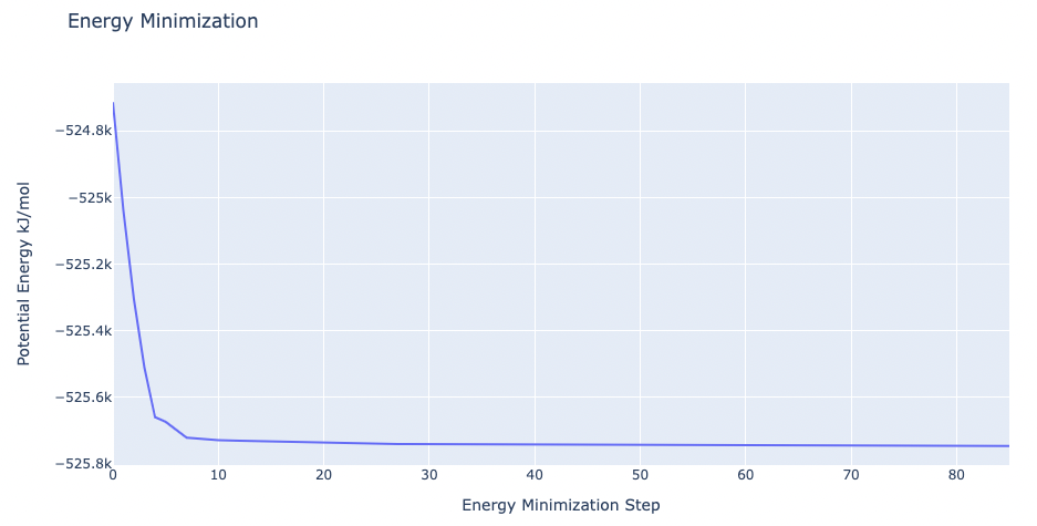
Energetically minimize the system
Energetically minimize the mutated protein till reaching a desired potential energy.
Step 1: Creating portable binary run file for energy minimization
Step 2: Energetically minimize the dummy atoms till reaching a force of 100 kJ/mol*nm.
Step 3: Checking energy minimization results. Plotting energy by time during the minimization process.
Building Blocks used:
Grompp from biobb_gromacs.gromacs.grompp
Mdrun from biobb_gromacs.gromacs.mdrun
GMXEnergy from biobb_analysis.gromacs.gmx_energy
Step 1: Creating portable binary run file for energy minimization
Method used to run the energy minimization is a steepest descent, with a maximum force of 100 kJ/mol*nm^2, and a minimization step size of 1fs. The maximum number of steps to perform if the maximum force is not reached is 10,000 steps. The previously generated FREEZE group is used to keep the system frozen except for the dummy atoms.
Please note that as previously described, for the stateA (forward transition, Isoleucine to Alanine mutation), as there are no dummies, the energy minimization is omitted and the energy minimization step is skipped.
# Grompp: Creating portable binary run file for dummy atoms energy minimization
from biobb_gromacs.gromacs.grompp import grompp

#### State B (Mut->WT) ####

# Create prop dict and inputs/outputs
output_tpr_min = 'em.tpr'

prop = {
    'gmx_lib' : gmxlib,
    'mdp':{
        'integrator' : 'steep',
        'emtol': '100',
        'dt': '0.001',
        'nsteps':'10000',
        'nstcomm': '1',
        'nstcalcenergy': '1',
        'freezegrps' : 'FREEZE',
        'freezedim' : "Y Y Y"
    },
    'simulation_type': 'minimization'
}

# Create and launch bb
grompp(input_gro_path=output_pdb2gmxB_gro,
       input_top_zip_path=output_pmxtopB_top_zip,
       input_ndx_path=output_ndx,
       output_tpr_path=output_tpr_min,
       properties=prop)
Step 2: Running Energy Minimization
Running energy minimization using the tpr file generated in the previous step.
# Mdrun: Running minimization
from biobb_gromacs.gromacs.mdrun import mdrun

# Create prop dict and inputs/outputs
output_min_trr = 'emout.trr'
output_min_gro = 'emout.gro'
output_min_edr = 'emout.edr'
output_min_log = 'emout.log'

# Create and launch bb
mdrun(input_tpr_path=output_tpr_min,
      output_trr_path=output_min_trr,
      output_gro_path=output_min_gro,
      output_edr_path=output_min_edr,
      output_log_path=output_min_log)
Step 3: Checking Energy Minimization results
Checking energy minimization results. Plotting potential energy by time during the minimization process.
# GMXEnergy: Getting system energy by time
from biobb_analysis.gromacs.gmx_energy import gmx_energy

# Create prop dict and inputs/outputs
output_min_ene_xvg = 'min_ene.xvg'
prop = {
    'terms':  ["Potential"]
}

# Create and launch bb
gmx_energy(input_energy_path=output_min_edr,
          output_xvg_path=output_min_ene_xvg,
          properties=prop)
import plotly.graph_objs as go

# Read data from file and filter energy values higher than 1000 kJ/mol
with open(output_min_ene_xvg, 'r') as energy_file:
    x, y = zip(*[
        (float(line.split()[0]), float(line.split()[1]))
        for line in energy_file
        if not line.startswith(("#", "@"))
        if float(line.split()[1]) < 1000
    ])

# Create a scatter plot
fig = go.Figure(data=go.Scatter(x=x, y=y, mode='lines+markers'))

# Update layout
fig.update_layout(title="Energy Minimization",
                  xaxis_title="Energy Minimization Step",
                  yaxis_title="Potential Energy kJ/mol",
                  height=600)

# Show the figure (renderer changes for colab and jupyter)
rend = 'colab' if 'google.colab' in sys.modules else ''
fig.show(renderer=rend)
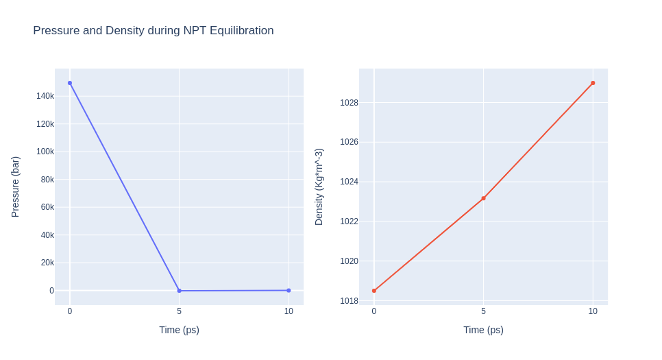
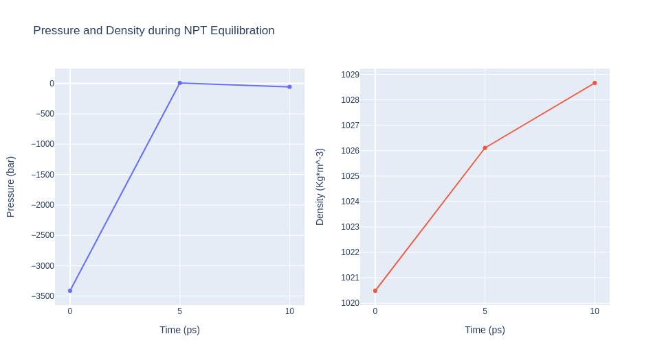
Equilibrate the system (NPT)
Equilibrate the protein system in NPT ensemble (constant Number of particles, Pressure and Temperature).
Step 1: Creating portable binary run file for system equilibration
Step 2: Equilibrate the protein system with NPT ensemble.
Step 3: Checking NPT Equilibration results. Plotting system pressure and density by time during the NPT equilibration process.
Building Blocks used:
Grompp from biobb_gromacs.gromacs.grompp
Mdrun from biobb_gromacs.gromacs.mdrun
GMXEnergy from biobb_analysis.gromacs.gmx_energy
Step 1: Creating portable binary run file for system equilibration (NPT)
The npt type of the molecular dynamics parameters (mdp) property contains the main default parameters to run an NPT equilibration with protein restraints (see GROMACS mdp options):
integrator = md
dt = 0.001
nsteps = 10000
pcoupl = Parrinello-Rahman
pcoupltype = isotropic
tau_p = 1.0
ref_p = 1.0
compressibility = 4.5e-5
refcoord_scaling = com
gen_vel = no
In this particular example, the default parameters will be used: md integrator algorithm, a time step of 2fs, 5,000 equilibration steps, and a Parrinello-Rahman pressure coupling algorithm.
Please note that for the sake of time this tutorial is only running 10ps of NPT equilibration, whereas in the original example the simulated time was 100ps.
# Grompp: Creating portable binary run file for system equilibration
from biobb_gromacs.gromacs.grompp import grompp

#### State A (WT->Mut) ####

# Create prop dict and inputs/outputs
output_tprA_eq = 'eqA_20ps.tpr'

prop = {
    'gmx_lib' : gmxlib,
    'mdp':{
        'nsteps':'10000',
        'nstcomm' : '1',
        'dt':'0.001',
        'nstcalcenergy' : '1'
    },
    'simulation_type': 'free'

}

#Create and launch bb
grompp(input_gro_path=output_pdb2gmxA_gro,
       input_top_zip_path=output_pmxtopA_top_zip,
       output_tpr_path=output_tprA_eq,
       properties=prop)


#### State B (Mut->WT) ####

# Create prop dict and inputs/outputs
output_tprB_eq = 'eqB_20ps.tpr'

prop = {
    'gmx_lib' : gmxlib,
    'mdp':{
        'nsteps':'10000', # 10000 steps x 1fs (timestep) = 10ps
        'dt':'0.001', # 1 fs of timestep, to properly equilibrate dummy atoms
        'nstcomm' : '1',
        'nstcalcenergy' : '1'
    },
    'simulation_type': 'free'
}
#Create and launch bb
grompp(input_gro_path=output_min_gro,
       input_top_zip_path=output_pmxtopB_top_zip,
       output_tpr_path=output_tprB_eq,
       properties=prop)
Step 2: Running NPT equilibration
# Mdrun: Running equilibration
from biobb_gromacs.gromacs.mdrun import mdrun

#### State A (WT->Mut) ####

# Create prop dict and inputs/outputs
output_eqA_trr = 'eqoutA.trr'
output_eqA_gro = 'eqoutA.gro'
output_eqA_edr = 'eqoutA.edr'
output_eqA_log = 'eqoutA.log'

# Create and launch bb
mdrun(input_tpr_path=output_tprA_eq,
      output_trr_path=output_eqA_trr,
      output_gro_path=output_eqA_gro,
      output_edr_path=output_eqA_edr,
      output_log_path=output_eqA_log)

#### State B (Mut->WT) ####

# Create prop dict and inputs/outputs
output_eqB_trr = 'eqoutB.trr'
output_eqB_gro = 'eqoutB.gro'
output_eqB_edr = 'eqoutB.edr'
output_eqB_log = 'eqoutB.log'

# Create and launch bb
mdrun(input_tpr_path=output_tprB_eq,
      output_trr_path=output_eqB_trr,
      output_gro_path=output_eqB_gro,
      output_edr_path=output_eqB_edr,
      output_log_path=output_eqB_log)
Step 3: Checking NPT Equilibration results
Checking NPT Equilibration results. Plotting system pressure and density by time during the NPT equilibration process.
# GMXEnergy: Getting system pressure and density by time during NPT Equilibration
from biobb_analysis.gromacs.gmx_energy import gmx_energy

#### State A (WT->Mut) ####

# Create prop dict and inputs/outputs
output_eqA_pd_xvg = 'eqA_PD.xvg'
prop = {
    'terms':  ["Pressure","Density"]
}

# Create and launch bb
gmx_energy(input_energy_path=output_eqA_edr,
          output_xvg_path=output_eqA_pd_xvg,
          properties=prop)

#### State B (Mut->WT) ####

# Create prop dict and inputs/outputs
output_eqB_pd_xvg = 'eqB_PD.xvg'
prop = {
    'terms':  ["Pressure","Density"]
}

# Create and launch bb
gmx_energy(input_energy_path=output_eqB_edr,
          output_xvg_path=output_eqB_pd_xvg,
          properties=prop)
Please note the information shown by the next plots increases with the time simulated, and are included as a reference for more complex calculations.
import plotly.graph_objs as go
from plotly.subplots import make_subplots

# Read pressure and density data from file
with open(output_eqA_pd_xvg,'r') as pd_file:
    x, y, z = zip(*[
        (float(line.split()[0]), float(line.split()[1]), float(line.split()[2]))
        for line in pd_file
        if not line.startswith(("#", "@"))
    ])

trace1 = go.Scatter(
    x=x,y=y
)
trace2 = go.Scatter(
    x=x,y=z
)

fig = make_subplots(rows=1, cols=2, print_grid=False)
fig.append_trace(trace1, 1, 1)
fig.append_trace(trace2, 1, 2)

fig.update_layout(
    height=500,
    title='Pressure and Density during NPT Equilibration',
    showlegend=False,
    xaxis1_title='Time (ps)',
    yaxis1_title='Pressure (bar)',
    xaxis2_title='Time (ps)',
    yaxis2_title='Density (Kg*m^-3)'
)

# Show the figure (renderer changes for colab and jupyter)
rend = 'colab' if 'google.colab' in sys.modules else ''
fig.show(renderer=rend)
import plotly.graph_objs as go
from plotly.subplots import make_subplots

# Read pressure and density data from file
with open(output_eqB_pd_xvg,'r') as pd_file:
    x, y, z = zip(*[
        (float(line.split()[0]), float(line.split()[1]), float(line.split()[2]))
        for line in pd_file
        if not line.startswith(("#", "@"))
    ])

trace1 = go.Scatter(
    x=x,y=y
)
trace2 = go.Scatter(
    x=x,y=z
)

fig = make_subplots(rows=1, cols=2, print_grid=False)
fig.append_trace(trace1, 1, 1)
fig.append_trace(trace2, 1, 2)

fig.update_layout(
    height=500,
    title='Pressure and Density during NPT Equilibration',
    showlegend=False,
    xaxis1_title='Time (ps)',
    yaxis1_title='Pressure (bar)',
    xaxis2_title='Time (ps)',
    yaxis2_title='Density (Kg*m^-3)'
)

# Show the figure (renderer changes for colab and jupyter)
rend = 'colab' if 'google.colab' in sys.modules else ''
fig.show(renderer=rend)
Free Energy Simulation
Alchemical transition (thermodynamic integration) free energy estimation approach is used with GROMACS: free energy is switched on, the initial lambda is chosen as zero, and delta-lambda (per MD step) is set such that at the end of the simulation lambda is at 1 (1 / nsteps). The dhdl files (dH/dl) written as a result will contain the work values required to perform these transitions.
Step 1: Creating portable binary run file to run the free energy simulation.
Step 2: Run short MD simulation of the protein system.
Building Blocks used:
Step 1: Creating portable binary run file to run a free energy simulation
The free_energy type of the molecular dynamics parameters (mdp) property contains the main default parameters to run an free energy simulation (see GROMACS mdp options):
integrator = md
dt = 0.002 (ps)
nsteps = 5000
free_energy = yes
init_lambda = 0
delta_lambda = 0.0002
sc-alpha = 0
sc-sigma = 0.3
In this particular example, the default parameters will be used: md integrator algorithm, a time step of 2fs, a total of 5,000 md steps (10ps), all with the free energy flag turned on, with an intial lambda of 0 and a delta lambda of 0.00002.
Please note that for the sake of time this tutorial is only running 10ps of NPT equilibration, whereas in the original example the simulated time was 100ps.
# Grompp: Creating portable binary run file for thermodynamic integration (TI)
from biobb_gromacs.gromacs.grompp import grompp

#### State A (WT->Mut) ####

# Create prop dict and inputs/outputs
output_tprA_ti = 'tiA.tpr'

prop = {
    'gmx_lib' : gmxlib,
    'mdp':{
        'nsteps':'5000',
        'free_energy' : 'yes',
        'init-lambda' : '0',
        'delta-lambda' : '2e-4',
        'sc-alpha' : '0.3',
        'sc-coul' : 'yes',
        'sc-sigma' : '0.25'
    },
    'simulation_type': 'free'
}

# Create and launch bb
grompp(input_gro_path=output_eqA_gro,
       input_top_zip_path=output_pmxtopA_top_zip,
       output_tpr_path=output_tprA_ti,
       properties=prop)

#### State B (Mut->WT) ####

# Create prop dict and inputs/outputs
output_tprB_ti = 'tiB.tpr'

prop = {
    'gmx_lib' : gmxlib,
    'mdp':{
        'nsteps':'5000',
        'free_energy' : 'yes',
        'init-lambda' : '0',
        'delta-lambda' : '2e-4',
        'sc-alpha' : '0.3',
        'sc-coul' : 'yes',
        'sc-sigma' : '0.25'
    },
    'simulation_type': 'free'
}

# Create and launch bb
grompp(input_gro_path=output_eqB_gro,
       input_top_zip_path=output_pmxtopB_top_zip,
       output_tpr_path=output_tprB_ti,
       properties=prop)
Step 2: Running free energy simulation
# Mdrun: Running equilibration
from biobb_gromacs.gromacs.mdrun import mdrun

#### State A (WT->Mut) ####

# Create prop dict and inputs/outputs
output_tiA_trr = 'tiA.trr'
output_tiA_gro = 'tiA.gro'
output_tiA_edr = 'tiA.edr'
output_tiA_log = 'tiA.log'
output_tiA_dhdl = 'tiA.xvg'

# Create and launch bb
mdrun(input_tpr_path=output_tprA_ti,
      output_trr_path=output_tiA_trr,
      output_gro_path=output_tiA_gro,
      output_edr_path=output_tiA_edr,
      output_log_path=output_tiA_log,
      output_dhdl_path=output_tiA_dhdl)

#### State B (Mut->WT) ####

# Create prop dict and inputs/outputs
output_tiB_trr = 'tiB.trr'
output_tiB_gro = 'tiB.gro'
output_tiB_edr = 'tiB.edr'
output_tiB_log = 'tiB.log'
output_tiB_dhdl = 'tiB.xvg'

# Create and launch bb
mdrun(input_tpr_path=output_tprB_ti,
      output_trr_path=output_tiB_trr,
      output_gro_path=output_tiB_gro,
      output_edr_path=output_tiB_edr,
      output_log_path=output_tiB_log,
      output_dhdl_path=output_tiB_dhdl)
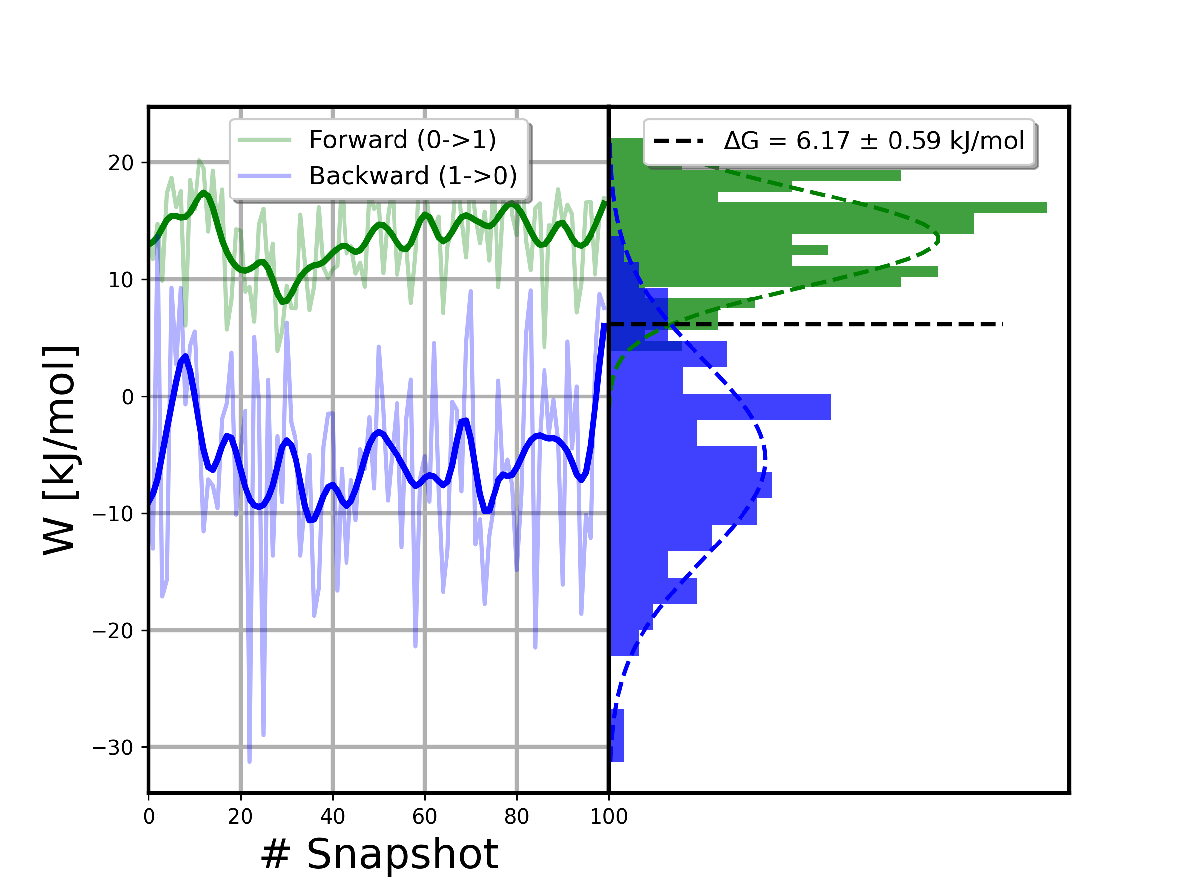
Free Energy Estimation
The Fast Growth TI approach relies on Jarzynski’s equality (when transition is performed in one direction only) or on the Crooks Fluctuation Theorem or the Bennett Acceptance Ratio (when the transitions are performed in both directions).
Workflow-generated results should be used if a minimum number of transitions are calculated. In this particular case, as the tutorial is just computing 1 transition (forward + reverse), the number of work values computed are not enough to extract the free energy. Instead, we will use values taken from a real run of the snase example that can be found in the pmx web page.
Step 1: Gathering together all the generated dhdl files (work values required to perform the transitions).
Step 2: Compute the free energy using Jarzynski’s equality, Crooks Fluctuation Theorem and Bennett Acceptance Ratio with pmx.
Building Blocks used:
Pmxanalyse from biobb_pmx.pmxbiobb.pmxanalyse
Step 1: Gathering together all the generated dhdl files
Gathering together all the generated dhdl files (work values required to perform the transitions). To be used as input for the final pmx free energy estimation.
# Gathering together all the generated dhdl files (work values required to perform the transitions)
# from the free energy simulations.
# To be used as input for the final pmx free energy estimation.

#### State A (WT->Mut) ####

zf = zipfile.ZipFile('dhdlsA.zip', mode='w')

for file in os.listdir(os.getcwd()):
    if file.endswith("A.dhdl.xvg"):
            zf.write(file)
zf.close()

#### State B (Mut->WT) ####

zf = zipfile.ZipFile('dhdlsB.zip', mode='w')

for file in os.listdir(os.getcwd()):
    if file.endswith("B.dhdl.xvg"):
            zf.write(file)
zf.close()
Step 2: Compute the free energy estimation
Compute the free energy using Jarzynski’s equality, Crooks Fluctuation Theorem and Bennett Acceptance Ratio with pmx.
# pmx analyse: analyze_dhdl command from pmx package

# Import module
from biobb_pmx.pmxbiobb.pmxanalyse import pmxanalyse

# Create prop dict and inputs/outputs

# Workflow-generated results should be used if a minimum number of transitions are calculated.
#state_A_xvg_zip = 'dhdlsA.zip'
#state_B_xvg_zip = 'dhdlsB.zip'

# In this particular case, as the tutorial is just computing 1 transition (forward + reverse),
# values taken from a real run of the snase example will be used instead.
state_A_xvg_zip = 'pmx_tutorial/dhdlA.zip'
state_B_xvg_zip = 'pmx_tutorial/dhdlB.zip'

output_result = 'pmx.txt'
output_work_plot = 'pmx.plots.png'

prop = {
    'reverseB' : True,
}

#Create and launch bb
pmxanalyse(input_a_xvg_zip_path=state_A_xvg_zip,
        input_b_xvg_zip_path=state_B_xvg_zip,
        output_result_path=output_result,
        output_work_plot_path=output_work_plot,
        properties=prop)
from IPython.display import Image
Image(filename=output_work_plot)
Output files
Important Output files generated:
output_result (pmx.txt): Final free energy estimation. Summary of information got applying the different methods.
output_work_plot (pmx.plots.png): Final free energy plot of the Mutation free energy pipeline.
Questions & Comments
Questions, issues, suggestions and comments are really welcome!
GitHub issues:
BioExcel forum: